Developer Blog - Solving Maxwell's Equations on Unstructured Meshes with SYCL and ComputeCpp
02 August 2018
Ayesha Afzal and Christian Schmitt are based at Friedrich-Alexander-Universität and part of a team working on the "HighPerMeshes" research project, a collaborative research project funded by German Ministry of Education and Research (BMBF).
The project team decided to use SYCL to develop the code for their research because it allowed them to write modern C++ code that can be deployed to a range of heterogeneous hardware.


In our research project HighPerMeshes, physicists use them to simulate nanoantennas and interferences within different materials. Our goal is to provide them with a technology that enables the implementation of simulation codes in a simpler and more productive fashion, while at the same time allowing them to deploy to different target devices and accelerators.
We decided to use SYCL to analyze and re-write a set of example code to solve Maxwell's equations because it allowed us to develop using standard C++, target a wide range of hardware, and gave us the opportunity to accelerate the code on this hardware.
To make the complex structures more like those in the real-world, we use unstructured meshes made up of tetrahedrons. As a drawback, unstructured meshes require irregular memory accesses and this makes them harder to program and parallelize than, for example, stencil codes on regular grids. As the numerical method, we use the Discontinuous Galerkin (DG) method in which each tetrahedron carries a number of so-called nodal points that are the basis for all computations. One advantage of the DG method is that computations can be done in parallel for all the nodal points. However, since the nodal points refer to physical coordinates, one correction step is required where values of corresponding nodal points are normalized using the so-called numerical flux. For the time integration, we use a fourth order, five stages low-storage Runge-Kutta scheme that has proven to be very efficient for this class of application, meaning computations need to be done five times per time step.
Starting from the original C code, we removed all references to external libraries used for handling of the mesh, including MPI used for parallelization. The original code consisted of three kernels to compute the numerical flux and the equation system's right-hand side on the surface of each mesh element, then inside each element, and finally to do the Runge-Kutta time integration step. We fused the two kernels that deal with the flux to make use of the data locality.
Additionally, we can have short and meaningful expressions in our code, such as
So, the program's structure looks like the following:
Overall, our SYCL-based implementation is significantly shorter and much easier to read and understand than the original code, and consequently less prone to programming errors. Additionally, we are able to easily evaluate the code not only on standard CPUs, but also on GPUs. In this work, we focused on the programmability and portability aspect of SYCL and did not research any potential impact on performance improvements we can apply to our code. There are many optimizations possible, such as avoiding scattered memory operations caused by the array-of-structs memory layout we are currently using, and taking care that all buffers are properly aligned and padded, to improve memory access times. Furthermore, we need to check which optimizations need to be applied for GPUs.
The project team decided to use SYCL to develop the code for their research because it allowed them to write modern C++ code that can be deployed to a range of heterogeneous hardware.
Christian has written the following post about their project and how the team used SYCL to make it a success.
Christian Schmitt Ayesha Afzal
Solving Maxwell's Equations on Unstructured Meshes with SYCL and ComputeCpp
Maxwell's equations form the foundation for electric, optical, and radio technologies, and thus are widely used in research and engineering.
We decided to use SYCL to analyze and re-write a set of example code to solve Maxwell's equations because it allowed us to develop using standard C++, target a wide range of hardware, and gave us the opportunity to accelerate the code on this hardware.
To make the complex structures more like those in the real-world, we use unstructured meshes made up of tetrahedrons. As a drawback, unstructured meshes require irregular memory accesses and this makes them harder to program and parallelize than, for example, stencil codes on regular grids. As the numerical method, we use the Discontinuous Galerkin (DG) method in which each tetrahedron carries a number of so-called nodal points that are the basis for all computations. One advantage of the DG method is that computations can be done in parallel for all the nodal points. However, since the nodal points refer to physical coordinates, one correction step is required where values of corresponding nodal points are normalized using the so-called numerical flux. For the time integration, we use a fourth order, five stages low-storage Runge-Kutta scheme that has proven to be very efficient for this class of application, meaning computations need to be done five times per time step.
Starting from the original C code, we removed all references to external libraries used for handling of the mesh, including MPI used for parallelization. The original code consisted of three kernels to compute the numerical flux and the equation system's right-hand side on the surface of each mesh element, then inside each element, and finally to do the Runge-Kutta time integration step. We fused the two kernels that deal with the flux to make use of the data locality.
The next step was to recover the semantics of computations. We replaced scalar variables that, for example represented three-dimensional vectors, with appropriate types. Additionally, these types feature overloaded mathematical operators and functions and this allowed us to represent coordinates and vector-valued data much more intuitively, e.g.:
// buffer for coordinates of nodal points per mesh element
cl::sycl::buffer<coord_t, 2> b_node_coords(cl::sycl::range<2>mesh_elements, nodal_points_per_element);

// buffers for magnetical and electrical fields for nodal points per element
cl::sycl::buffer<real3_t, 2> b_H(cl::sycl::range<2>mesh_elements, nodal_points_per_element);
cl::sycl::buffer<real3_t, 2> b_E(cl::sycl::range<2>mesh_elements, nodal_points_per_element);
Additionally, we can have short and meaningful expressions in our code, such as
real3_t const fluxH = dH - dot_product(normal, dH) * normal - cross_product(normal, dE);
real3_t const fluxE = dE - dot_product(normal, dE) * normal + cross_product(normal, dH);
Here, coord_t and real3_t are simply vectors of three doubles. A lot of geometrical information on the mesh is needed for the computations, e.g., neighborhood relations between elements and their faces for the exchange of the numerical flux. Naturally, we implemented the geometric data as SYCL buffers using our data types to use them inside the kernels. However, a large portion of this data has to be calculated first, as the mesh file only stores physical coordinates of vertices and a mapping from vertices to elements. This preparatory work does not need to be accelerated (in fact, it is hard to parallelize and the speedup gained is negligible), so we do this sequentially on the host CPU and only initialize and use the SYCL queue much later.
// declaration of SYCL buffers for mesh and data
// initialization of mesh data structures
// computation of neccessary mesh information and data initialization

#if defined USE_CPU
auto selector = cl::sycl::cpu_selector{};
#elif defined USE_GPU
auto selector = cl::sycl::gpu_selector{};
#endif
auto device = selector.select_device();

cl::sycl::queue queue(selector);
for (size_t timestep = 0; timestep < timesteps; ++timestep) {
    for (size_t runge_kutta_stage = 1; runge_kutta_stage <= 5; ++runge_kutta_stage) {
        queue.submit([&](cl::sycl::handler &cgh) {
            // accessors ...
            cgh.parallel_for<class mw_surfacevolume>(cl::sycl::nd_range<1>mesh_elements, 32, [=](cl::sycl::nd_item<1> itm) { ... });
        };
        queue.submit([&](cl::sycl::handler &cgh) {
            // accessors ...
            cgh.parallel_for<class mw_rk>(cl::sycl::nd_range<1>mesh_elements, 32, [=](cl::sycl::nd_item<1> itm) { ... });
        };
    }
}
Overall, our SYCL-based implementation is significantly shorter and much easier to read and understand than the original code, and consequently less prone to programming errors. Additionally, we are able to easily evaluate the code not only on standard CPUs, but also on GPUs. In this work, we focused on the programmability and portability aspect of SYCL and did not research any potential impact on performance improvements we can apply to our code. There are many optimizations possible, such as avoiding scattered memory operations caused by the array-of-structs memory layout we are currently using, and taking care that all buffers are properly aligned and padded, to improve memory access times. Furthermore, we need to check which optimizations need to be applied for GPUs.
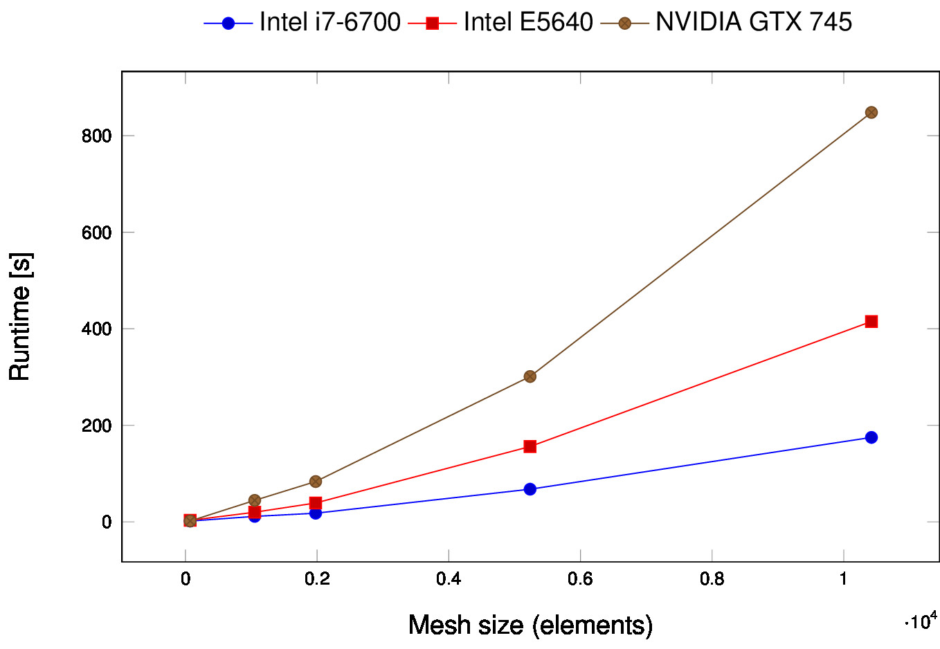
However, to simply get an impression of the resulting performance, we ran exactly the same code on a number of different devices, i.e., an Intel Core i7-6700, an Intel Xeon E5640, and a low-end NVIDIA GPU (GTX 745) for mesh sizes ranging from 72 to 10k elements.
As a conclusion, we are very satisfied with how easy it was to implement the code with SYCL, but need to do further investigations on how to write performance-optimal code. If you are interested in reading a detailed explanation and discussion using software complexity metrics, please have a look at our published research paper.
Codeplay Software Ltd has published this article only as an opinion piece. Although every
effort has been made to ensure the information contained in this post is accurate and
reliable, Codeplay cannot and does not guarantee the accuracy, validity or
completeness of this information. The information contained within this blog
is provided "as is" without any representations or warranties, expressed or implied.
Codeplay Sofware Ltd makes no representations or warranties in relation to
the information in this post.